3. Processing physiological data
There are a few common processing steps often performed when working with physiological data:
We have already seen that peakdet.operations has functions to perform
a few of these steps, but it is worth going into all of them in a bit more
detail:
3.1. Visual inspection
One of the first steps to do with raw data is visually inspect it. No amount of
processing can fix bad data, and so it’s good to check that your data quality
is appropriate before continuing. Plotting data can be achieved with
plot_physio():
>>> from peakdet import load_physio, operations
>>> data = load_physio('ECG.csv', fs=1000.0)
>>> ax = operations.plot_physio(data)
>>> ax.set_xlim(0, 10)  # doctest: +SKIP
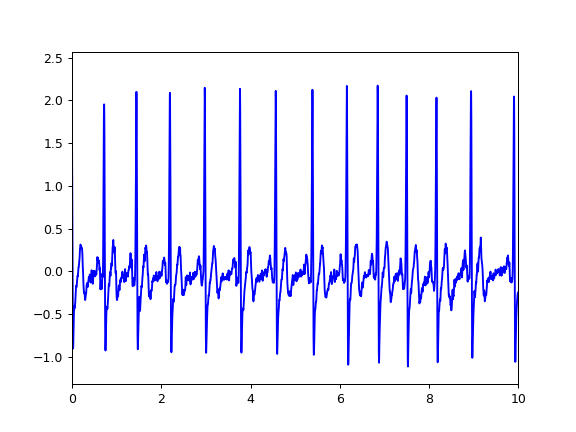
For now this will simply plot the raw waveform, but we’ll see later how this function has some added benefits.
3.2. Interpolation
Raw data can often be collected at a sampling rate above what is biologically
meaningful. For example, human respiration is relatively slow, so acquiring it
at, for example, 250 Hz is often more than sufficient; when it is acquired at a
higher rate it can be quite noisy. In this case, we might want to interpolate
(or decimate) the data to a lower sampling rate, which can be done with
interpolate_physio():
>>> data = load_physio('RESP.csv', fs=1000.)
>>> print(data)
Physio(size=24000, fs=1000.0)
>>> data = operations.interpolate_physio(data, target_fs=250.)
>>> print(data)
Physio(size=6000, fs=250.0)
Note that the size of the data decreased by a factor of four (24000 to 6000), the same as the decrease in sampling rate.
Data can also be upsampled via interpolation, though care must be taken in interpreting the results of such a procedure:
>>> data = load_physio('PPG.csv', fs=25.0)
>>> print(data)
Physio(size=24000, fs=25.0)
>>> data = operations.interpolate_physio(data, target_fs=250.0)
>>> print(data)
Physio(size=240000, fs=250.0)
3.3. Temporal filtering
Once our data is at an appropriate sampling rate, we may want to apply a
temporal filter with filter_physio(). This function
supports lowpass, highpass, bandpass, and bandstop filters with user-specified
frequency cutoffs. First, let’s take a look at our interpolated PPG data:
>>> ax = operations.plot_physio(data)
>>> ax.set_xlim(0, 10)  # doctest: +SKIP
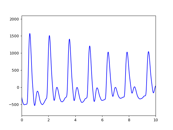
If we’re going to do peak detection, it would be great to get rid of the venous pulsations in the waveform to avoid potentially picking them up. If we apply a lowpass filter with a 1.0 Hz cutoff we can do just that:
>>> data = operations.filter_physio(data, cutoffs=1.0, method='lowpass')
>>> ax = operations.plot_physio(data)
>>> ax.set_xlim(0, 10)  # doctest: +SKIP
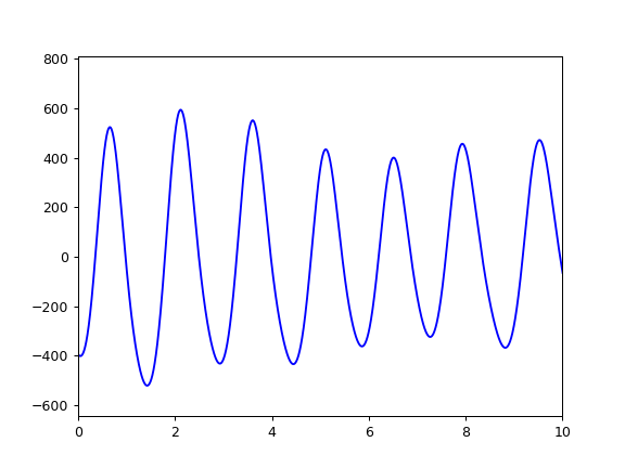
Filter settings are highly dependent on the data, so visually confirming that the filter is performing as expected is important!
3.4. Peak detection
Many physiological processing pipelines requiring performing peak detection on
the data (e.g., to calculate heart rate, respiratory rate, pulse rate). That
process can be accomplished with peakfind_physio():
>>> data = operations.peakfind_physio(data, thresh=0.1, dist=100)
>>> data.peaks[:10]
array([ 164,  529,  901, 1278, 1628, 1983, 2381, 2774, 3153, 3486])
>>> data.troughs[:10]
array([ 356,  732, 1111, 1465, 1817, 2205, 2603, 2989, 3330, 3677])
The peaks and troughs attributes mark
the indices of the detected peaks and troughs in the data; these can be
converted to time series by dividing by the sampling frequency:
>>> data.peaks[:10] / data.fs
array([ 0.656,  2.116,  3.604,  5.112,  6.512,  7.932,  9.524, 11.096,
       12.612, 13.944])
>>> data.troughs[:10] / data.fs
array([ 1.424,  2.928,  4.444,  5.86 ,  7.268,  8.82 , 10.412, 11.956,
       13.32 , 14.708])
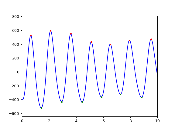
Once these attributes are instantiated, subsequent calls to
plot_physio() will denote peaks with red dots and troughs
with green dots to aid visual inspection:
>>> ax = operations.plot_physio(data)
>>> ax.set_xlim(0, 10)  # doctest: +SKIP